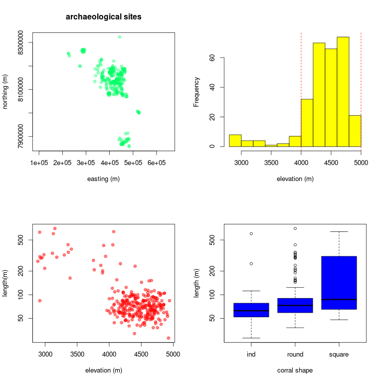
Basical statistical programming using R

R is an open-source statistical computing language and perhaps the most widely used platform among researchers. This is quickly becoming the case for archaeologists too. Despite it's analytical power, R is also suprisingly simple and intuitive. At it's most basic level, it can serve as a simple calculator for addition, subtraction, multiplaction, and division. From there, the sky is the limit. R can be used to perform matrix algerbra, statistical analysis, simulation, mapping, visualization, Bayesian computation, and the list goes on. This tutorial will introduce you to a few foundational skills including basic calculation, data tables, summary statistics, and plotting. For example, you will learn how to quickly find the mean and standard deviation for a set of numerical values and visualize data trends using graphical plots. Here are some examples of the graphical visualizations that you will produce in this tutorial:
plots

Installation

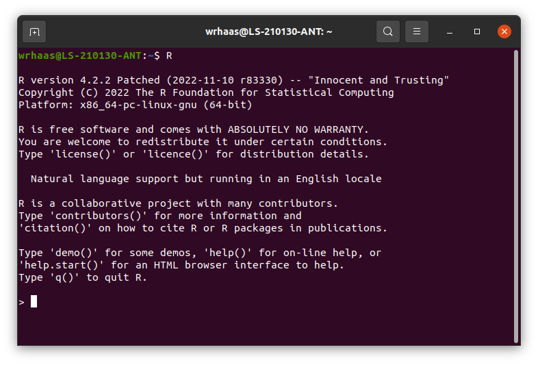
To complete this tutorial, you must install R on your computer. R is available for Windows, Mac, and Linux operating systems. Follow the installation instructions provided on the R website where you will click the CRAN link under the Download menu item. Select any link from the long list of download locations. I usually select the one that is geographically closest to me. It doesn't matter which you choose. Installation instructions will vary by operating system and version. This tutorial is based on R version 4.2.2 as implemented in linux Ubuntu 20.04 operating system. These system details may entail small–sometimes frustrating–differences for users working with Mac or Windows operating systems.

For Ubuntu users (Windows and Mac users, ignore), the standard R installation only runs in Terminal, which does not allow you to save your script. Although running R in Terminal can be useful for quick calculations, it's limited for more involved coding that requires editing over multiple sessions. To create a scripting component, you need to install packages called, emacs and ess. Emacs is simple text editing software that is commonly used in programming. ESS (emacs speaks statistics) is an add-on package for emacs that allows R and emacs to communicate. These can be easily installed via Terminal as follows:

sudo apt install emacs
sudo apt install ess

Opening R

Use your favorite method to open R. Typically this involves double-clicking on the R icon on your Desktop or other location. However, I prefer to open a command line terminal and enter R. This may seem silly, but it is actually the fastest way to open the software once you get used to it. Whatever approach you take, the following screen will appear (or something like it depending on your operating system):

This screen shows the R console. The console is where calculations are performed.

Basic calculation

Now that you have an R console open, let's perform some basic calculations.

Enter, 4+4. Be sure to enter the command by hitting the Enter key. You will see that R performs this basic calculation like any calculator.
Enter, 4+4*2/(3+6)-5. Again, you get the result for this basic arithmetic according to standard order of operations.
Enter, 3^5. R handles exponentiation (i.e., raising to a power) calculations easily with the carat symbol (^). The carat symbol is usually located at or near the number 6 on your keyboard.
Now create a variable called x to represent the number 4 as follows:
```
x<-4
```
This says x=4. In R computing language <- is the equal sign used when storing variables.
Enter, x. You should see the number 4 returned in your console.
Enter, x+25. You should see the number 29 returned in your console. In this simple way, R can perform simple algabreic calculations of virtually any complexity.

Vectors

R can also work with collections of numbers, called vectors.

In R console, enter a vector called y with 10 values as follows:
```
y<-c(4,6,2,3,6,7,8,2,1,3)
```
The c() portion of this line is a combine function that combines the entities entered between the parentheses. Each data point is separated by a comma. More information about functions will be presented below.
Enter y to verify that you've properly stored the vector. You should see the numbers returned on the screen.
Suppose that these numbers represent a series of counts (e.g., the number of structures per archaeological site), and for some reason you want to augment each value by 1. Enter y+1. You will see that 1 has been added to all numbers.
Enter y. Notice that the numbers have returned to their original values. This is because you did not store your updated vector.
To store the updated variable, enter y<-y+1. This says that y equals y + 1.
Enter y, and you will now see that all y values have been updated.
Create a second vector called z with 10 new numbers that you randomly choose.
Enter z to verify your vector.
Suppose that y and z are the lengths and widths of 10 objects–perhaps archaeological sites. Store the product of y and z as a variable called a as follows:
```
a<-y*z
```
Enter a to verify the result. You should see 10 numbers that reflect the product of the x and y vectors.
Vectors can also contain text. Create a variable called site that stores the letters A–K. When entering text data in R, the text should be in quotes to avoid confusion with variable names (e.g., we don't want R to confuse our site area variable, a with a site called "A"). You could accomplish this as follows:
```
site<-c("A","B","C"...)
```
But here's a shortcut:
```
site<-LETTERS[1:10]
```
Note that you can do something similar with number sequences such that 1:10 will return the numbers 1–10 in sequence. Try it without storing the number sequence. I.e., enter
```
1:20
```
Subsetting: there may be times you would like to access some subset of a vector such as the first value, the last value, or the fifth value, for example. To do that, you enter your vector name followed by brackets that indicate which values you want to return. For example, if you just want the first area value, enter a[1], and the first area value will be returned.
Return the fifth entry be typing
```
a[5]
```
Return the second through the eighth entries by typing
```
a[2:8]
```

Functions

Functions are tools for quickly performing calculations on datasets. For example, we can use functions to calculate the average, minimum, or maximum value for a set of numbers. In R, functions are expressed as the function name followed by input data in parentheses. For example, the mean function is expressed as mean(x), which finds the mean for vector, x. R has thousands of functions for data analysis. We'll work through a few commonly used functions. You can find other functions as needed with simple web searches.

Use the mean function to calculate the mean of your site areas as follows:
```
mean(a)
```
Use the min function to calculate the mean of your site areas as follows:
```
min(a)
```
Now try passing a through the following commonly used functions: max, median, sd, and summary.
Getting help: enter, ?sd to open the help file for the sd function. A help file will appear. If you ever need information about a function, just open the function's help file by typing ? followed by the function name. You can close this help file in R Terminal by hitting the letter "q" (exiting the help file may vary by system. Consult Google as needed).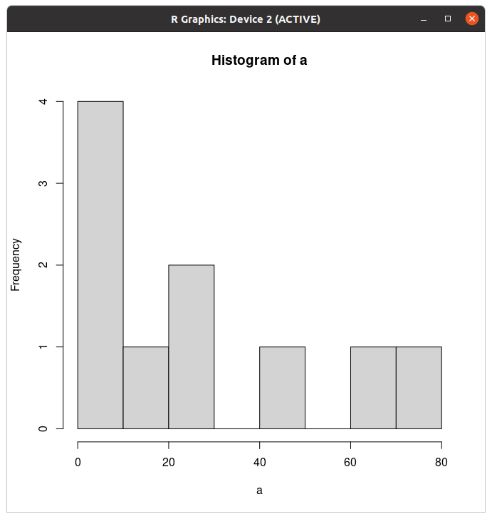
Functions can also be used for simple graphical applications. Try,
```
hist(a)
```
This is the histogram function, and it produces a frequency plot of your data. It should look something like this:

Histograms offer useful visualizations of numerical data. You can quickly get a sense of the range of values and any trends.
Function arguments. Functions can be fed additional information, called arguments. Suppose we want to label the x axis of our histogram with a more meaningful label. We can add the xlab argument as follows:
```
hist(a, xlab="site area (sq. m)")
```
Note that arguments are separated by commas. Now your histogram should exhibit a relabled x axis.
Change the color of the bars to red by re-running the function and adding the argument, col="red". Tip: you can typically use your keyboard's up-arrow to recall a previous line of code so that you don't have to re-type code from scratch each time.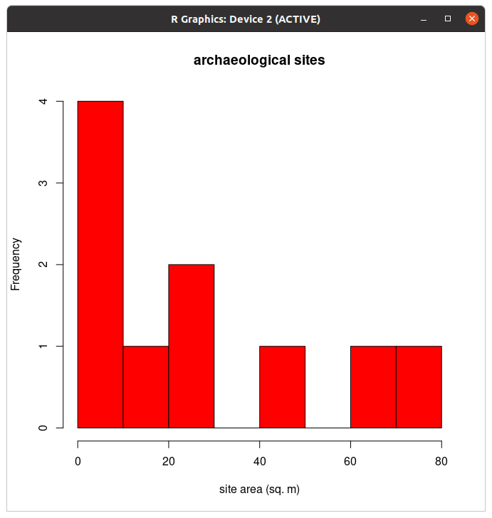
Change the title of the plot to "archaeological sites" by adding the argument called, main. Your plot should now look something like this:
Another common and useful plot function is the boxplot, or box-and-whisker plot. Boxplots are used to compare numerical datasets. Compare your y and z values using the boxplot function as follows:
```
boxplot(y,z)
```
Yet another common and useful plot function is the scatter plot, which is simply plot. Scatterplots are used to evaluate relationships between two numerical variables. Use the plot function to see if there is a relationship between y and z as follows:
```
plot(y,z)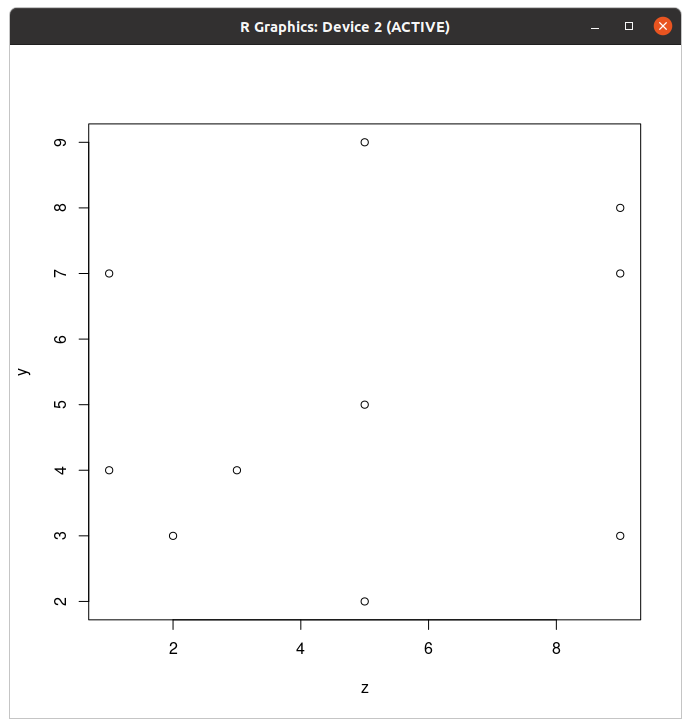
```
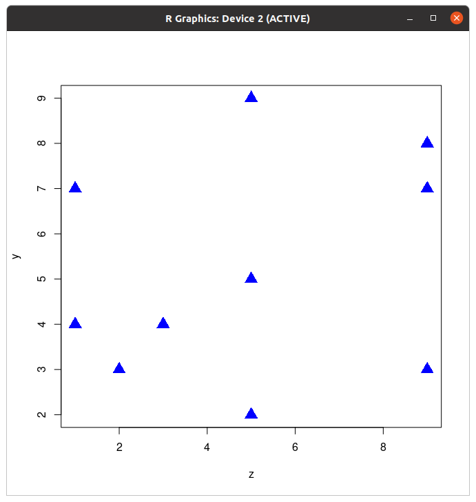
You should get something like this:
Change the dot colors to blue using the col argument as described above; change the dots to triangles using the argument, pch=17; and double their size with the argument, cex=2.
pch stands for "plot character." Do a google search for "R pch" to see what the plot character codes are. cex stands for "character expansion" and specifies a multiplier for how much you want to increase the the size of plot characters. For example, cex=2 increases the size of the character by a factor of 2—the size is doubled. Your plot should look something like this now:

Exporting graphics

Although graphics windows are useful for visualizing your data on the computer, they are not well formatted for printing or publication. To export properly formatted graphics, you can use the png function. This function allows you to precisely control the size and resolution of your graphical output so that it is perfectly formatted for publication. The function assumes some knowlege of how computer graphics work. These details will not be discussed here, but they are addressed in the graphics tutorial using Gimp. See that tutorial for technical details toward understanding graphics.

Enter the following png command into your console, customizing the path name to specify where you would like to store the image on your computer:
```
png("/home/username/SomeFolder/TutorialStatisticalProgramming/plot.png",width=4,height=4,units="in",res=300,pointsize=10)
```
Note that this directory syntax is specific to linux. It will differ for Windows and Mac users who should consult Google for the correct syntax.
What this code says is, create an image file called "plot.png" at the specified location on your computer, and make that image 4 inches high x 4 inches wide at a resolution of 300 pixels per inch. 300 pixels per inch is a standard resolution for pubication. The "pointsize" argument sets the default text size to 10 pt, which is a common font size for publication graphics.
When you hit enter, nothing will happen. This is because what you've done is opened an invisible plot window in the background, which is ready to accept your plot.
Re-enter the plot function from step 11 of the Functions section above. Again, this can be done quickly using your keyboard's up arrow.
Enter the device off function to close your plot window as follows:
```
dev.off()
```
Again...nothing will happen...apparently. Use your file browser to navigate to the directory where you placed the png file. You should find "plot.png" there. Double click it to open the image in the default image viewer. You should now see a nicely formatted plot that you could add to a word processing document (see LibreOffice Word Processing tutorial).

Data frames

Vectors are useful when dealing with few data points. As the number of data points or vectors increases, it becomes useful to use data frames. Data frames refer to data tables, which can be stored as variables in R just like vectors and individual quantities.

Create a dataframe using your site, y, z, and a vectors using the data.frame function as follows:
```
data.frame(site,length=y,width=z,area.m=a)
```
Note that we can specify column names for each variabl using the "=" sign. For example, here we've specified that "length" is the column name for our variable, y.
Now store the data frame as a variable called df by preceding the last line of code with df<-.
Enter df to return your data frame. Now you have a nice data frame to work with. Let's see how to work with data frames.
Subsetting: There are time when you would like to work with a specific portion of your data frame. As with vectors, you can subset data frames using brackets. However, you must specify both the row and column numbers that you wish to subset. Row and column numbers are separated by a comma. Suppose you would like to view only the area value for site D. Enter,
```
df[4,4]
```
You will see only the area value for site D, which is located in row 4, column 4, is returned.
Suppose you wish to return all information associated with site D. Enter,
```
df[4,]
```
Leaving the column term blank indicates that all columns should be returned. You should see just the column 4 values.
The same can be done for rows. Try, for example,
```
df[,4]
```
, which will return all area values–that is, all values in the fourth column of the data frame.
Another convenient method for retreiving data frame columns is to use the $ term to specify a column name within a data frame. For example, try
```
df$length
```
Now lets put this to use. Suppose you would like to visually summarize the length values in your data frame with a histogram. Enter,
```
hist(df$length)
```

Data import

Often we would like to import large datasets such as those that are created in spreadsheets. Although it is possible to import an number of data formats into R, the most widely used is the Comma Separated Value (csv) format. csv files are easily created using standard spreadsheet software such as LibreOffice Calc (see spreadsheet tutorial) or Microsoft Excel. In this section you will import a largdataset of archaeological sites. The sites will be explained in the final section of this tutorial. For now, just know that you are importing a dataset in which each line in the table represents an archaeological site, and each column represents some attribute associated with those sites.

Import the data using the read.csv function, and store the data frame under the variable name, "data", as follows:
```
data<-read.csv("/home/yourname/folders/TutorialStatisticalProgramming/chaccus.csv")
```
Enter, data, to see your imported data table. Note that its a bit large an unwieldy.
Use the head function to inspect the first few lines of the data as follows:
```
head(data)
```
Make a simple map of the data locations by plotting the easting and northing values as follows:
```
plot(x=easting,y=northing,asp=1)
```
The asp = 1 term says to constrain the x and y axes to a 1:1 ratio because they are the same units as is the case for most geographic maps. You should see a simple map of your data points that looks as follows:
You would like to know how many sites there are in this dataset, which can be assessed by asking how many lines are in the table. Get your answer with the nrow function as follows:
```
nrow(data)
```
You can now use any of the functions described in the previous sections to assess your data. Try, for example,
```
mean(data$length)
```
to return the average length of the chaccu features.

Scripting

Ubuntu users

To create an R script, you have to first create an R file, and open it in emacs. Typically, I do this by entering the following in Terminal:
```
emacs SomeFileName.R &
```
The first time you open emacs, an introductory screen will appear. Check the "Never show it again" box, and click the "Dismiss startup screen" link. You will now see a blank document. This is where you write your script.
Type x<-4.
Pass that line of code from your script to the R console by hitting Ctrl+enter on your keyboard. The first time you do this, you will be prompted to start a directory. Just hit enter to accept the default. A console screen will appear with the code that you passed to it. Your emacs script and R console will look as follows:

Windows and mac users

Open R and create a new text file using the File menu bar like you would in any other software.
Type x<-4.
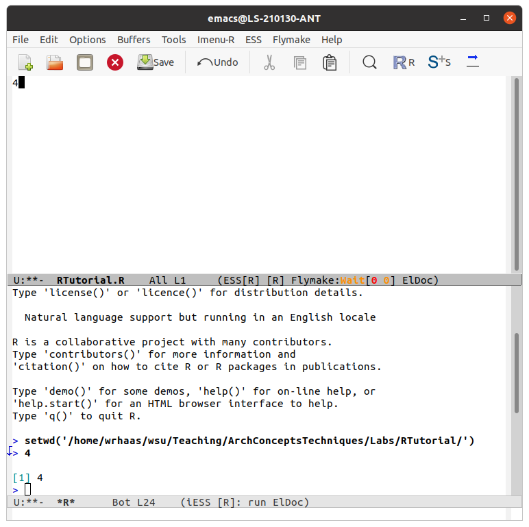
Pass that line of code from your script to the R console by hitting Windows + r or Apple + r on your keyboard.
You can now enter and save R script in an R file and pass code to the console with a simple keystroke. Save and close the file using the menu buttons in emacs or R, as the case may be.

Exercise: An archaeological analysis

You will now bring all methods together to script an archaeological analysis using R code. You will evaluate a hypothesis for a series of archaeological features that were recently discovered in satellite imagery. These mysterious features are V-shaped stone walls that occur in the Andean highlands of South America. Here's an example of one of these archaeological features as seen in satellite imagery:
chaccu satellite

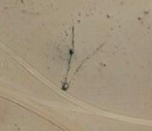
Archaeologists have documented hundreds of these. One hypothesis suposes that they served as animal trapping features used by Indigenous communities to cooperatively hunt large mammals, likely vicuña. This hypothesis anticipates that the traps are located in vicuña habitat, which occurs between 4000-5000 meters above sea level (masl). Your goal is to test this prediction—to determine if these features are located between 4000–5000 masl as the communal hunting hypothesis predicts. Follow the instructions below referring back to the methods above as needed. Your graphics will look something like this,
plots
but feel free to add your own stylistic twists.

Create a new R script document called "chaccu.R".
In your new script, import the csv file called "chaccus.csv", and store these data as a variable called, "sites".
Show the first five lines of the table using the head function. Note that each line of the data frame represents a site.
Determine how many sites are in the table using the nrow function. How many sites are in the dataset?
Make a simple map of the site locations using the plot function with the east variable as the x value and north variable as y value. Be sure to include the asp=1 term to make sure the x and y axes are equivalently scaled. Do you observe any patterning in the geographies of the sites?
Given that you are trying to understand the elevation of the sites, do you see any data columns that indicate elevation? Return the elevation data using the $ function as described in the data frame section of this tutorial. It's difficult to make any sense of so many values just by looking at them. We need a better way to visualize and summarize the data.
Now inspect the elevation of the archaeological features by creating a histogram of the "elev.m" variable using the hist function and generating summary statistics using the summary function. Note that the units are meters above sea level.
Recall that the model predicts that the traps fall between 4000–5000 meters above sea level. Add a vertical red line to your histogram at 4000 m using the abline function as follows:
```
abline(v=4000,col="red",lty=2)
```
The "v" term indicates that the line should be vertical. The lty term refers to line type. A value of 2 produces a dashed line. And, of course, "col" refers to color.
repeat the previous command at 5000 m. What do you observe in the historgram? Do the data conform to the prediction?
Update your plot code so that the x axis is labeled, "elevation (m)" and the title is blank (main="").
Use the png function to export a png image called "ElevHist.png" that is 5 x 5 inches at 300 DPI and 10 pt font.
You should observe that the data largely conform to the prediction but also that there is a cluster of values that occur below 4000 m. You note that a different, larger species of camelid called the guanaco lives at that elevation. From that hypothesis, you predict that the low elevation traps should be larger to accomodate the larger animals.
Evaluate this new hypothesis using the plot function with elevation as the predictor variable (x axis) and length as the response variable (y axis). Does there appear to be any relationship?
Update your plot code so that the x axis is labeled, "elevation (m)", the y axis is labeled "length (m)", and the title is blank.
Use the png function to export a png image called "ElevLength.png" that is 5 x 5 inches at 300 DPI and 10 pt font.
You further observe that there are two different "corral" shapes—round and square, which is recorded in the "corral.shape" variable. Use the boxplot function to determine whether site length differs by "corral" shape. Your boxplot code will be a little different here compared to how you executed the code before. This time, you will express your continuous variable (elevation) as a function of the categorical variable as follows:
```
boxplot(sites$length~sites$corral.shape)
```
Note that the tilde (~) means "as a function of." So this code says, make a boxplot where site length varies as a function of corral shape. Does there seem to be a relationsip?
You should provisionally see a relationship, but it's a bit difficult to tell because the values are "squished" toward the bottom of the plot. A nice trick for spreading out your data is to logarithmically scale your axis. Do this by adding a log="y" term to your plot as follows:
```
boxplot(sites$length~sites$corral.shape,log="y")
```
Notice that the y axis scale in now non-linear. Is the pattern any clearer?
Update your boxplot code so that the x axis is labeled, "corral shape"; the y axis is labeled "length (m)"; and title is blank.
Use the png function to export a png image called "ShapeLength.png" that is 5 x 5 inches at 300 DPI and 10 pt font.
You realize that you have no idea how big these features are. Do they span centimeters? Meters? Kilometers? You should probably verify that the size of the features is reasonable given the hypothesis. Inspect site size by creating a histogram of the "length" variable using the hist function and generating summary statistics using the summary function. Note that the units of the length variable are meters. What do you observe? Do these seem like reasonably sized features given the hypothesis?
Update your histogram code so that the x axis is labeled, "length (m)" and the title reads, "suspected animal traps".
Use the png function to export a png image called "LengthHist.png" that is 5 x 5 inches at 300 DPI and 10 pt font.
You've now analyzed the animal-trap hypothesis using R statistical computing language. Well done. What can you conclude? Do the data support the predictions? Embed your graphics in LibreOffice document with figure captions (see LibreOffice tutorial), and draft a one-paragraph conclusion that references your graphics.